Piezoelectric Transducers convert between electrical energy and sound energy. Piezoelectric Actuators, specifically, convert periodic electrical signals into vibrations. Near-Field Acoustic Levitation is a phenomenon close to the surface of an acoustic source where the complex constructive and destructive interference pattern generates a persistent outward force.

This project leverages said phenomenon by integrating an array of piezoelectric transducers into a stage that levitates and drives a silicon wafer or “puck” on air. The greater goal is to deterministically control (closed-loop) the puck/silicon wafer through an arbitrary trajectory.

By sampling the control space of different amplitude and phase shift patterns I expect to determine a series of mappings from amplitude and phase shift patterns to elemental translational and rotational displacements (and velocities too, possibly).

Currently approaching the learning phase, this portfolio post is a high-level cursor over several implementation aspects and decisions. I aim to outline the mechanical design, the electrical schematics and components tested and selected, the layered of the control architecture, and the data collection pipeline.

Mechanical Design

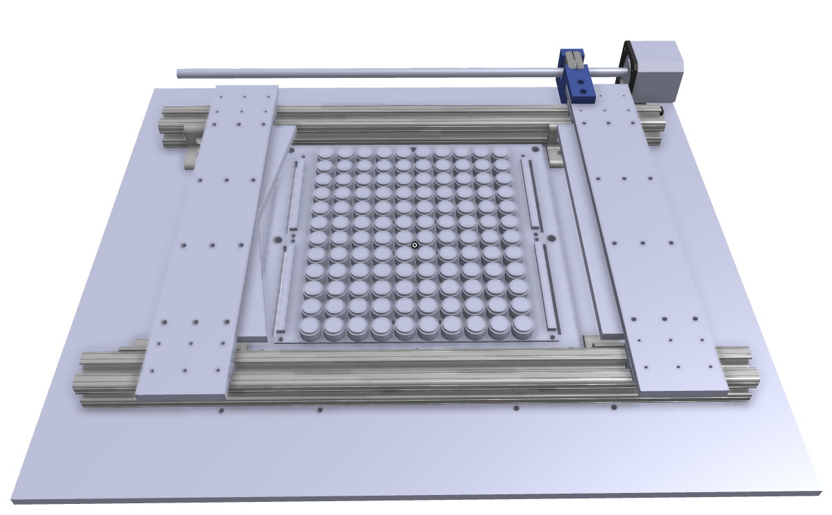
The objective here was to build up a bed of acoustic transducers arrayed in a grid as with pixels in a digital image. This bed would be embedded on a bigger stage, which also features a vision system, and a pair of actuatable guide walls.

The bed was designed as a set of 4 printed circuit boards, each laying out a 5 x 6 array of densely-packed transducers connected to their respective signed header-pin connectors. Butted-together in a pattern of four corners and mounted on the same base plate, the 4 transducer PCBs form a 10x12 grid with banks of header pins along two sides. The header pins connect underneath to the bridging circuitry and drive electricals – described later.

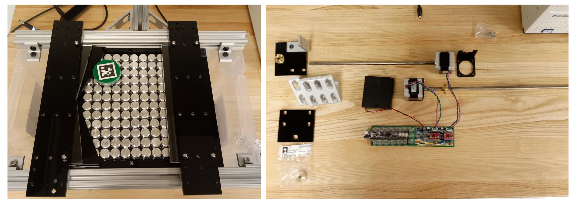
The actuatable guidewalls serve to re-center the puck in the data acquisition phase of the process. A vee-shaped contact feature on one guide wall, and straight contact feature on the other are actuated independently to come together, to engage with the puck wherever it may be in on the bed. In the resulting gripping action, the puck centered on the bed. A pair of aluminum 80-20 extrusion sections running the length of the stage act as the guide rails. Sections of PLA blocks, profiled to the slots of the aluminum extrusion and connected to the guide walls, act as guide blocks. Each guide is then actuated by a lead-screw and stepper motor tandem turning in a constrained nut.

The vision system features a RealSense D435i camera held in place above and pointing toward the bed. It’s job? To locate the puck and track its responses to different acoustic stimuli; as proxy limit switches, to determine the end of travel for the actuatable guide walls; and to trigger when the guidewalls should be actuated to center the puck.

Electrical Design and Components Selection

Each transducer would be connected to drive circuitry, each of which provides a periodic signal equal in frequency to the resonance of the transducer. Each signal, assuming symmetrical constant-frequency sinusoids, is characterized by its phase shift and amplitude providing two degrees of freedom for each acoustic actuator.

The Pui Audio UT21440KTTR ultrasonic actuators were selected over the MA40H1S-R (Murata), the MA40S4S (Murata), the H2KA300KA1CD00 (Unictron) and .. for a number of reasons: The 140 Vpp rating allowed for higher energy and more observable vibrations The emitting surface was already exposed and did not require sensitive modifications to access The through-hole mounting construction was easy to work with and fabricate for However, the less-than-desired large diameters dictated a more sparse packing density and reduced resolution of the grid. Also, the high voltage application required extra safety measures. Related heat concerns arose later in the process as well.

All in all, I investigated two electrical schematics each with a different control approach.

[Image: Bitbanging control signal]

The original idea was to control each of the 120 transducers with a uniquely assigned switching circuit. A 3.3V square wave originating from an assigned output pin of a microcontroller (PIC32) would trigger a low-side high voltage high-frequency gate driver through an optoisolator. The MCU would receive a bit-banging sequence as a list of 10 integers, one for each 10th of a time period. Then, in response to a timer-based interrupt triggering every 1/400kHz seconds, the digital output pins would toggle as desired by the bit-banging sequence.

I developed the firmware as two different programs: one to run on a “master” MCU and another to run on “slave” MCUs, with a “metronome” signal for synchronization and a serial bus for passing the bit-banging sequence through to respective MCUs. In summary: 120 GPIO pins across 4 PIC32 MCUs for the required 120 transducer signals.

[Image: Electrical Sigs,Screenshots from oscilloscope of bit-bangin, of opto-signal]

On the electrical side of things, I eventually zeroed in on the required components for the drive circuitry, generating a “high voltage” switching signal to a singular transducer. To extend this to 120 was intractable fabrication-wise (to say the least), so I pivoted away from the design that would limit the control signal to less-than-ideal square-waves, that would limit the voltage across the transducers to 70 Vpp instead of the full 140, that would reduce the control space to only phase shifts, and that would complexify the harder-to-test low-level control system.

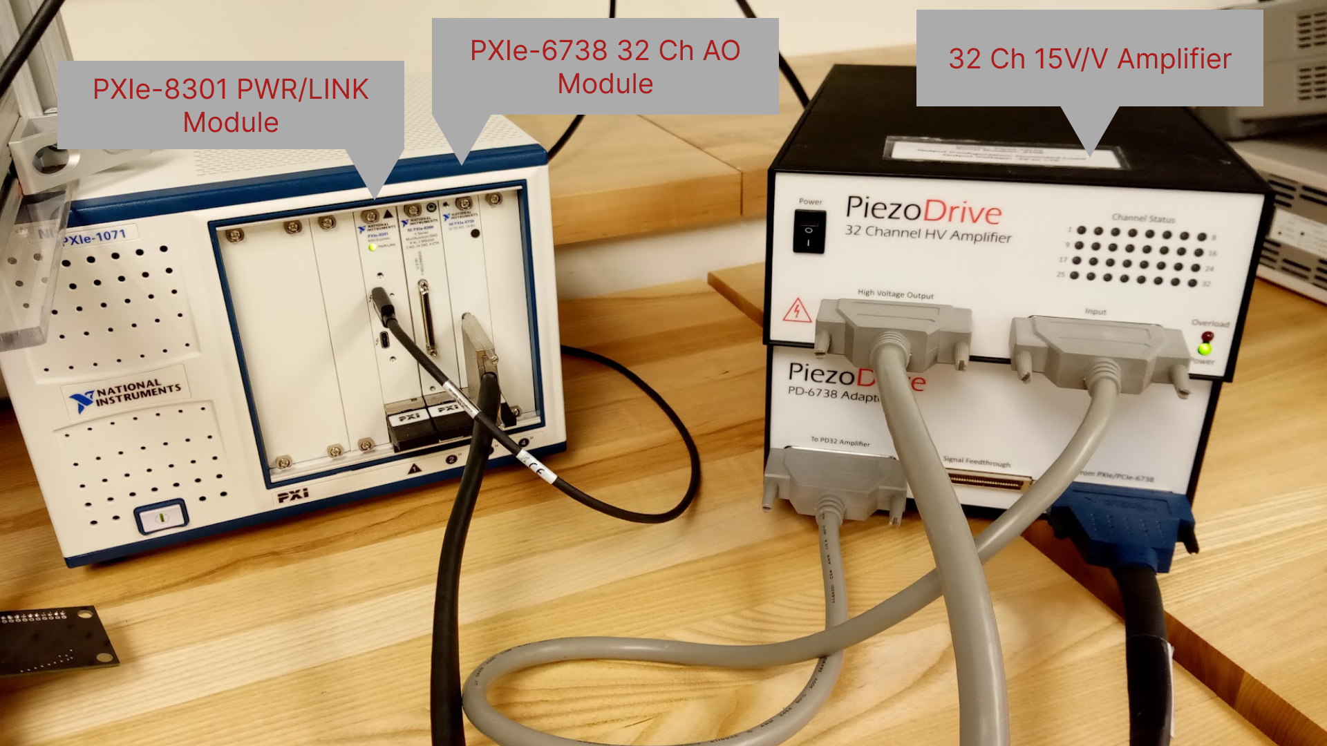
The second and eventual approach was to use the existing National Instruments lab equipment: in particular, a single 32 channel analog output module controlled/commanded through LabVIEW. This greatly simplified the PCB design requirements and avoided an otherwise arduous soldering job ahead.

30 channels output for 120 transducers

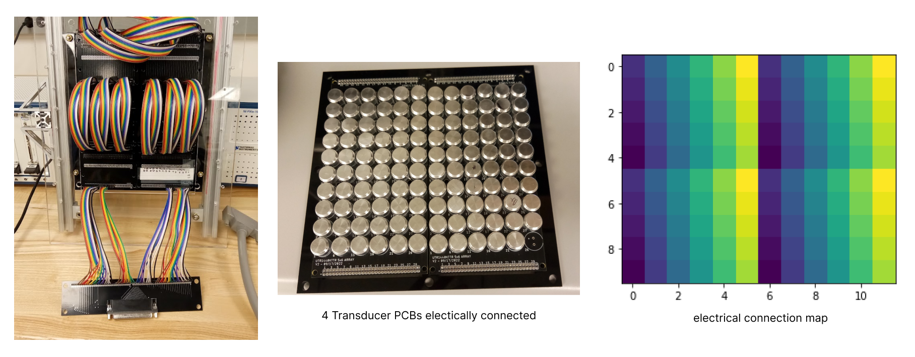
The key to unlocking and using the 32 channel analog output module for the 120 singly addressable transducers was the size of the puck. And seeing that the puck roughly covered a 3X3 grid on the bed of transducers, I needed to only control a 5x5 grid of transducers at a time. And so I could share a single channel with 4 transducers sparsely-distanced from each other. And so I could make do with 30 channels altogether, each purposely tied to a transducer location for each of the 4 Transducer PCBs. And so I would have to compensate with a more intricate vision program accompanied by an Output Control Generator algorithm.

[Image: Vision processing flow]

The vision program was developed to

• crop the captured image,
• rectify the perspective distortion,
• divide the region of interest (ROI) into a 10 x 12 grid
• detect the puck and locate the grid location of its centroid
• and generate a surrounding subgrid for use in the Output Control Generator algorithm

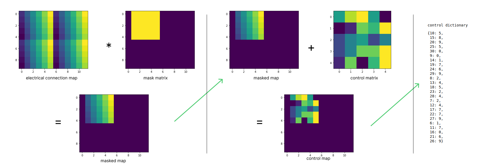
The Output Control Generator algorithm encodes the subgrid as a mask matrix, and convolves it as a mask over the mapping matrix to generate a masked mapping. The masked mapping combines with either control matrix to generate a control dictionary sent to the automated LabVIEW control.

(Terminology: map matrix, mask matrix, phase shift matrix, amplitude matrix, control matrix, masked map, subgrid)

Hardware and Software Organization

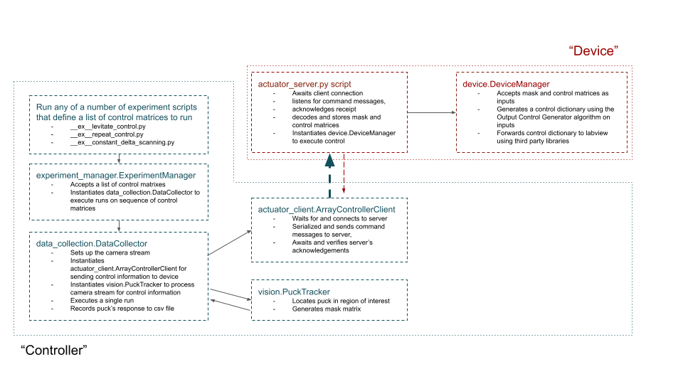
The software stack, largely a collection of python modules and scripts, was set up to be run across two separate computer systems and to facilitate communication between said systems and between said systems and their respective peripherals.

The NI apparatus was connected to a dedicated Windows PC, pre-installed with license-activated LabVIEW. The PC, the LabVIEW virtual instrument configured for the 32 Channel Analog output module, through to the breakout connector interface for the bed of arrays, and the device.py and actuator_server.py modules constitute the “device-side” of the architecture.

The “controller-side”, on the other hand, captures the vision system connected to the controller laptop, running any of a number of data collection, data processing or trajectory scripts.

The actuator_server.py and actuator_client.py provide the socket connection and API for communication across the controller-device divide. Both computer systems have to be on the same Local Area Network, and specify the same host IP address. Control Matrices and Mask Matrices are serialized on the “controller side”, and acknowledged and deserialized on the “device side”.

The device.py module encapsulates the output control generator algorithm and provides the utilities to combine the control matrices and mask matrices into a control dictionary to forward to the LabVIEW VI. Interfacing with labVIEW is handled by a combination of third party python libraries installed on the Windows PC: labview_automation and hoplite

The data_collection.py module configures the realsense camera stream, sends control inputs to the “device” and records the puck’s response to a csv file. The vision.py module collects together the pre- and post-processing operations involved in locating and tracking the puck. The experiment_manager.py module applies the data_collection sequence to a series of control_inputs. This then becomes the high-level utility for specifying different experimental ideas. The __ex__constant_detla_scanning.py, for example, use the experiment_manager.py module to investigate columnwise phase shifts.

Later – soon – a data_processing.py module will provide a framework to parse the csv file logs of the various data collection scripts, to re-visit and -visualize the puck’s varied responses to acoustic stimulus patterns, and to filter/order according to a given objective function.

Data Collection and Exploring the Control Space

A single “run” of the data collection phase sequentially:

1. Locates the puck
2. Begins recording the puck’s location and orientation with time stamps
3. Actuates the transducer by effecting a control dictionary based on the puck’s location/subgrid
4. Waits a specified run duration before stopping the transducers
5. Stops recording the puck’s movement
6. Then finally saves the run’s data to a specified csv file.

This template is repeated over and over – once for each pair of control matrices (ie a pair of one phase shift matrix and one amplitude matrix) This process of cycling through is currently set up to be manually triggered for each run, and to display a verification image that highlights the puck’s location on the bed of transducers and the subgrid to which the amplitude is applied.

Beyond building and controlling the hardware, exploring the vast control space is the next frontier, where the goal is to map the puck movements to control matrix combinations. All things being equal across all transducer units, I can reduce the control space of the “phase matrix” to all possible 5x5 grids matrices. Restricting the amplitude control to a binary input per unit, I can with similar reasoning reduce the control space of the “amplitude matrix” to 2^25 possibilities.

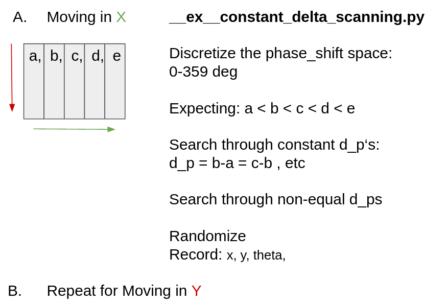
In the preliminary experiments, I guessed a set of reasonable patterns to try, and iterated from there. The __ex__constant_delta_scanning.py script implements an experiment of maintaining similar phase control to transducers along a column of the subgrid andex a constant phase shift from column to column.

ControlSpace

Next Steps

Results are yet inconclusive Next Steps? Q-learning and random sampling!